Generating Terrestrial Planets Pt.1

This is related to Semi-Empirical Stellar Equations. I have had some questions easily answered, and others which are difficult or impossible to get the kind of accuracy I want.

I’m going to order what I’ve learned by the order I am planning to use these equations, marking equations loosely based on empirical data with an asterisk, and double asterisks for things I’ve completely made up to simplify calculation.

  • Radius of Surface* (Rsurface):
    5500km mean, 1550km standard deviation
  • Density* [based on common rock types] (Dplanet):
    4.7g/cm3 mean, 0.55g/cm3 standard deviation
  • Volume [assumes a perfect sphere] (Vplanet):
    4/3 * π * Rsurface3
  • Mass (Mplanet):
    Dplanet * Vplanet
  • Surface Gravity (gsurface):
    6.673×10⁻¹¹Nm2kg-2 * Mplanet / Rsurface2
  • Surface Area [assumes a perfect sphere]:
    4 * π * Rsurface2
  • Atmospheric Pressure Reduction Rate** (Pr):
    Pr [unit: none] = -0.00011701572 [unit: s2 / m2] * gsurface
  • Atmospheric Halving Height** (hd):
    hd [unit: m-1] = ln(2) / Pr
  • Atmospheric Volume at Constant Pressure** (Vsim):
    (4/3 * π * (Rsurface + hd)3 – Vplanet) * 2
  • Surface Atmospheric Pressure (Psurface):
    Psurface [unit: kPa] = ???
  • Lowest Safe Orbital Height** (h0):
    h0 [unit: m] = ln(1.4×10⁻¹¹ / Psurface) / Pr
  • True Atmospheric Volume (Vatm):
    4/3 * π * (Rsurface + h0)3 – Vplanet

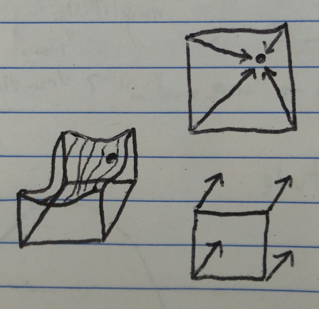
Vsim exists to support a simulation of an entire planet’s atmospheric contents using my simple fluid simulation mechanic. The magic constant used to calculated Pr is based on Earth’s atmosphere, it can be changed to set an exact “atmospheric height” while maintaining other properties of this simulation.

  • Atmospheric Pressure at Altitude** (Paltitude):
    Paltitude [unit: kPa] = Psurface * exp(Pr * maltitude) [Pr may be -Pr, I don’t remember]

This post is obviously incomplete, but it’s been a while since I posted anything here, and I felt like I should go ahead and share what I’ve been up to.

Semi-Empirical Stellar Equations

I’ve spent a lot of time trying to answer certain questions in astronomy, where I just want a rough approximation for the purpose of a simulation, and don’t need an exact answer. These are some of the equations I’ve come up with.

Yerkes Classes’ T/Mv Relations

These equations are shown as functions where x is temperature in Kelvin, and f(x) is absolute magnitude (visual). Most are valid from 2400 K to a little bit past 30000 K, the exceptions are noted. For the hypergiants and white dwarfs, the range is within an elliptical region, of which these functions define the major axis; for all others, they are a trend line along a Yerkes classification.

  • Hypergiants (0):
    f(x) = -8.9
  • Supergiants (Ia):
    f(x) = -0.00135x3 + 0.0233x2 + 0.0187x – 7.349
  • Supergiants (Ib):
    f(x) = 0.00329x3 – 0.0962x2 + 0.829x – 7.209
  • Bright Giants (II):
    f(x) = 0.00557x3 – 0.166x2 + 1.505x – 6.816
  • Giants (III):
    f(x) = 0.0135x3 – 0.373x2 + 3.019x – 7.233
  • Subgiants (IV):
    f(x) = -0.151x2 + 2.216x – 5.128 (4450-100000 K only)
  • Dwarfs (V):
    f(x) = 0.00193x5 – 0.0615x4 + 0.742x3 – 4.257x2 + 12.439x – 12.996 (note: this one is the least accurate)
  • Subdwarfs (VI):
    f(x) = 0.131x3 – 3.275x2 + 27.576x – 71.7 (3050-6000 K only)
  • White Dwarfs (VII):
    f(x) = 0.489x + 10.01 (4450-30000 K only)

Simple Conversions

  • Absolute Magnitude (visual) → Luminosity (solar luminosities):
    Lsun = 100 * exp(-0.944 * Mv)
    Accurate between 0-10 Mv. Probably continues accuracy relatively well.
  • Main Sequence Luminosity / Mass Relation:
    Lstar / Lsun = (Mstar / Msun)3.5
    Lstar = ( 3.68 * ln(Mstar) – 0.244 )e
    (The second equation applies to all stars.)
  • Mass / Lifetime Relation:
    Tyears = ( 23.4 – 2.68 * ln(Mstar) )e
    (This applies to all stars.)

Spectral filters are used to help classify stars. Ultraviolet, Blue, Visual, Red, and Infrared. Objects are listed in different indexes:

  • UV for the hottest objects (stellar remnants, galaxies)
  • BV (the majority of stars)
  • RI for the coolest (LTY “stars” and below)

Equations I no longer recommend

Provided for completeness, in case they are found to be useful.

  • Temperature (K) → Absolute Magnitude (visual):
    Mv = 35.463 * exp(-0.000353 * T)
    Roughly accurate between 2000-50000 Kelvin. Probably doesn’t continue accuracy at hotter temperatures. Previously this was at the top of this post, now I am not sure why (perhaps the simplicity). The Yerkes’ classifications are a better system.
  • B-V index (x) → Temperature (K):
    T = -772.2x3 + 3152x2 – 6893x + 9500
    Sorta accurate between 0-2. (This equation I am least comfortable with, and don’t plan to use.)

Grammar-Based Generation

To me, this is a new form of procedural generation. You declare specific rules for your desired content, and then a generator runs accordingly. I’ve only seen it used for text, but I’m sure the same technique works for anything. The simplest example is picking a random item from a list, and a slightly more complex version shows the power of defining a grammar:

grammar = {
  "first name": "Anna", "Belle", "John"
  "last name": "Brown", "Jameson", "Williams"
  "full name": "{first name} {last name}"
}

G(grammar, "full name") -- ex: Anna Williams

The syntax above is pseudocode for a generator I am working on. I plan to allow the use of a custom seed along with the generator so that you can do things like have uniquely generated people for a population, where only a lookup number needs to be stored (if you wish to remember a specific person).

It gets even more powerful when you make it possible to define multiple versions of the same grammar and use different ones depending on an object’s properties, and allow inline code within the grammars. Here’s an incomplete example based on my continuing efforts to build space games:

{
  "system name": {
    {
      props: { pulsar: true }
      "PSR {random(1000)}"
    }
    {
      props: { pulsar: false }
      "{Greek letter} {Latin name}"
      "{random(100)} {Latin genitive}"
      "{modern constellation} G{random(1000,9999)}.{random(1000,9999)}"
    }
  }
}

For this example, pulsars would get their traditional “PSR ###” names, while non-pulsars would get names based on differing classification methods.

I’m currently thinking about a game based on Aurora, but massively simplified and playable in-browser. Grammar-based content generation would play a very important role in this, from generating system names (as above) to NPC ship design.

References

Resources that helped me recognize the potential of grammars:


(Normally I would like to publish working code along with these posts, or some other form of useful data, but today we’re looking at a work-in-progress idea without even that much concrete form.)

Trying to Understand Noise

Perlin noise and simplex noise are the topics I keep coming back to, because I know they form the basis of a lot of procedurally generated content. All I knew about them to start with was give this function a value for 1 to 4 dimensions, and it will return a “random” value that is constant based on the input.

There is a somewhat ambiguous warning about passing integers “might” lead to a constant result. No, it will always be the same value at any integer. Turns out this is fundamental to how noise functions work:

graphic examples of how Perlin noise is constructed

One explanation I’ve read says that Perlin noise is essentially mixing dot products from 4 vectors from neighboring integers to the exact point you’ve chosen and 4 copies of a constant vector present at each of those “corners.” This is represented by the arrows in the above image.

A consequence of the constant vector at every integer value is that any integer will return the exact same value.

1D simplex noise is remarkably similar to a sine wave

Another explanation describes a noise function as mixed sine functions of differing amplitudes and frequencies. Looking at an output from 1-dimensional noise definitely can make it appear to be that simple, but it isn’t. I mention this idea for three reasons:

  1. It looks similar. This can help trying to visualize it.
  2. It is periodic, you do not have an infinite domain of values to choose from without repetition.
  3. Some terminology can still apply, such as adjusting the frequency or amplitude of noise, and depending on implementation, the range can be the same (or something easy like LÖVE‘s 0 to 1).
visual representation of properties of waves

Noise Usage

I have been trying to use noise for quite a while, with a lot of failure, mainly around not understanding the domain and range of the noise function. As of now, these are the things I’ve learned:

  • Period / Domain: There is a sample of (usually) 256 values used for the constant vectors, this defines the period before the noise function starts repeating. Keep this in mind combined with other adjustments to hide or avoid this repetition. (This is how I discovered the period of LÖVE’s implementation.)
  • Frequency: A higher frequency can be achieved by stretching the input, leading to quicker, more dramatic transitions.
  • Amplitude: This one feels kind of obvious, but with LÖVE, the output is 0 to 1, so that needs to be mapped to whatever range is desired.

Sources (aside from those linked in-article):

My apologies, but any other relevant sources at this time have been lost to the ages, with the possible exception of the source code to a demake of No Man’s Sky I have put some work into. I will revisit that at a later date.