I don’t understand lambda calculus

Update, 2024-10-11: Man, this is a garbage post. I was trying to get my thoughts out, but I have next to no clue what I was doing and don’t really understand it. You want to learn about Lambda Calculus? Go anywhere else. Sorry. >.<


I’m playing around in Minetest, and I have an idea. In order to execute this idea, I’m going to need a simple programming language. Asking Google… implementing a simple programming language

7 lines of code, 3 minutes: Implement a programming language from scratch
Sounds good! Ridiculously simple, fast, and gives us a fully usable language. (I would’ve understood brainfuck better..) Let’s see what this language looks like:

(λ v . e)   anonymous function with argument v and returning e
(f v)       call function f with argument v
(λ a . a)   example: identity function (returns its argument)

And the scary one:
(((λ f . (λ x . (f x))) (λ a . a)) (λ b . b))

Seems okay until I get to understanding that last example. If you’re curious about the steps I went through before I finally figured it out, here are my notes. I’m gonna skip to the good part:

(((λ f . (λ x . (f x))) (λ a . a)) (λ b . b))
two identity functions, let's name them I, & remove excess parenthesis
(λ f . (λ x . (f x))) I I
the syntax is still confusing me, let's make an "F" function
F(x) -> return (λ x . (f x))
F I I                          equivalent to ((F I) I)
substituting the function (identity) into our definition gives us
(λ x . (I x))                  which..is actually the same as the identity function
I(I)                           ..it all comes to returning the identity function

λ x . x

Now, at this point I’ve learned a few small tricks for my understanding, as well as how lambda calculus works in general.

Reduction

Solving a lambda calculus program is made of three (or 2.5) steps called reductions:

  • η-conversion (eta): Replace equivalent functions with simpler forms (λ x . f x) -> f
  • β-reduction (beta): Substitution (λ a . a) x -> x (essentially, THIS is solving it)
  • α-conversion (alpha): Rename conflicting names (λ a . a b) (λ a . a) -> (λ a . a b) (λ c . c)

References

This is where my journey ends for now. I started studying lambda calculus because of a desire to implement a simple programming language, but this will likely not satisfy my needs..at least not in this form. (Note: All resources are archived using the services linked to on Archives & Sources.)

Trying to Understand Noise

Perlin noise and simplex noise are the topics I keep coming back to, because I know they form the basis of a lot of procedurally generated content. All I knew about them to start with was give this function a value for 1 to 4 dimensions, and it will return a “random” value that is constant based on the input.

There is a somewhat ambiguous warning about passing integers “might” lead to a constant result. No, it will always be the same value at any integer. Turns out this is fundamental to how noise functions work:

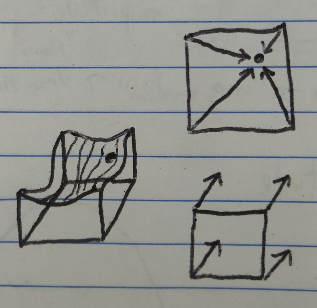
graphic examples of how Perlin noise is constructed

One explanation I’ve read says that Perlin noise is essentially mixing dot products from 4 vectors from neighboring integers to the exact point you’ve chosen and 4 copies of a constant vector present at each of those “corners.” This is represented by the arrows in the above image.

A consequence of the constant vector at every integer value is that any integer will return the exact same value.

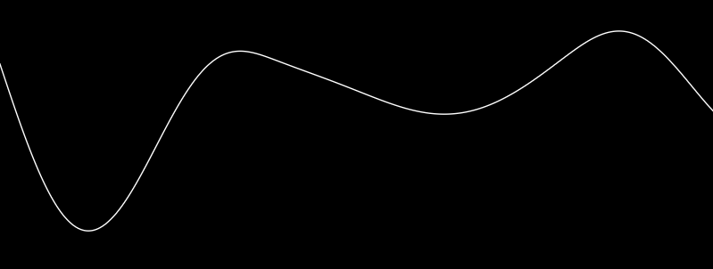
1D simplex noise is remarkably similar to a sine wave

Another explanation describes a noise function as mixed sine functions of differing amplitudes and frequencies. Looking at an output from 1-dimensional noise definitely can make it appear to be that simple, but it isn’t. I mention this idea for three reasons:

  1. It looks similar. This can help trying to visualize it.
  2. It is periodic, you do not have an infinite domain of values to choose from without repetition.
  3. Some terminology can still apply, such as adjusting the frequency or amplitude of noise, and depending on implementation, the range can be the same (or something easy like LÖVE‘s 0 to 1).
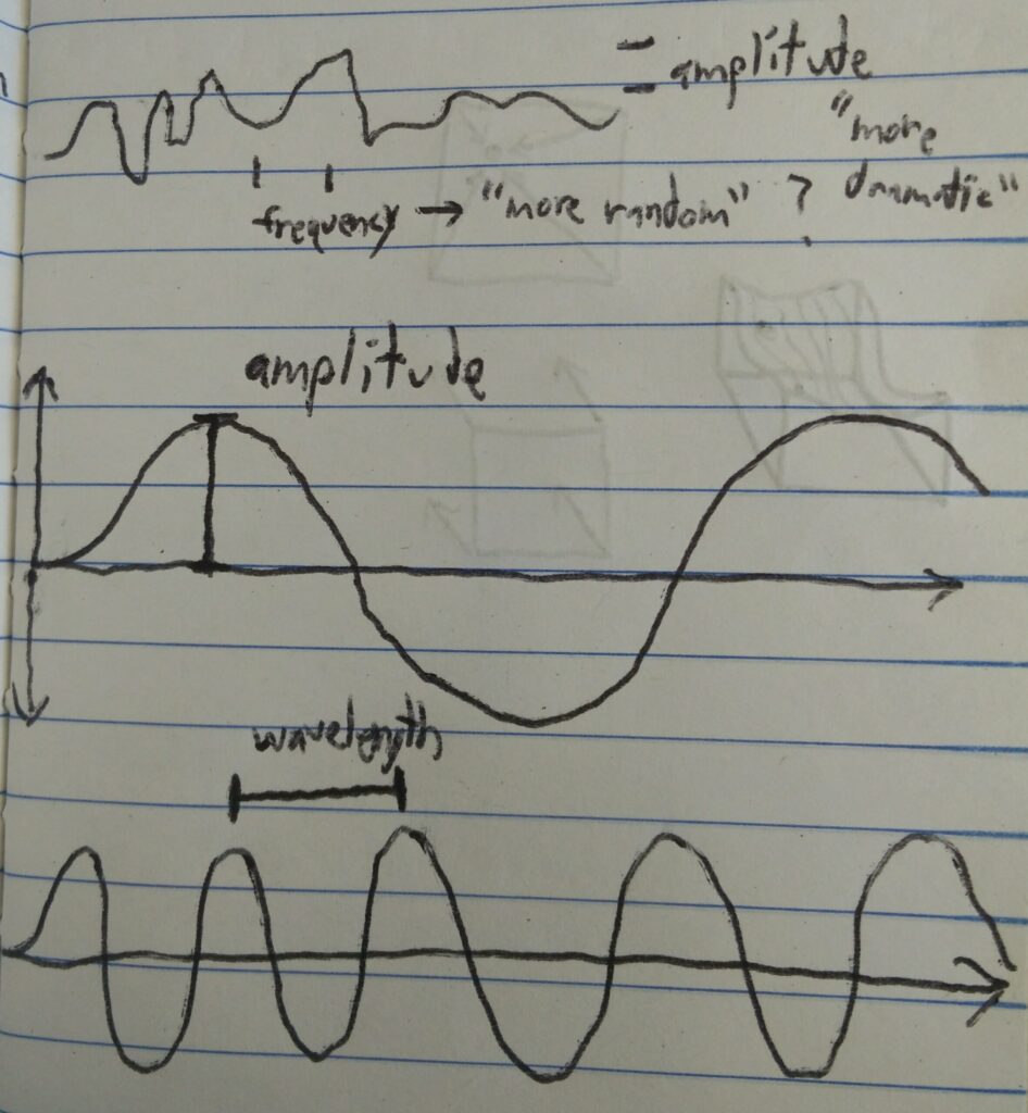
visual representation of properties of waves

Noise Usage

I have been trying to use noise for quite a while, with a lot of failure, mainly around not understanding the domain and range of the noise function. As of now, these are the things I’ve learned:

  • Period / Domain: There is a sample of (usually) 256 values used for the constant vectors, this defines the period before the noise function starts repeating. Keep this in mind combined with other adjustments to hide or avoid this repetition. (This is how I discovered the period of LÖVE’s implementation.)
  • Frequency: A higher frequency can be achieved by stretching the input, leading to quicker, more dramatic transitions.
  • Amplitude: This one feels kind of obvious, but with LÖVE, the output is 0 to 1, so that needs to be mapped to whatever range is desired.

Sources

(Skipping those linked to within the post. Note: All resources are archived using the services linked to on Archives & Sources.)

My apologies, but any other relevant sources at this time have been lost to the ages, with the possible exception of the source code to a demake of No Man’s Sky I have put some work into. I will revisit that at a later date.